
News
Direct answer: OEE is the share of planned production time a line spends making good product at its designed speed. It is three numbers multiplied, not one: Availability × Performance × Quality. A single OEE percentage tells you nothing until you know how each factor was measured — what counted as planned time, what ideal cycle time was used, and whether reworked boards counted as good. There is no universal “good OEE” percentage. The widely quoted 85% comes from one set of ideal-plant figures published in the 1980s, not from a standard, and a high-mix line with several changeovers a day will score below it for structural reasons. Read the three factors separately, and OEE becomes the fastest way to find which station is actually costing you output.
A supplier, a consultant or your own production report hands you a number: “our line runs at 72% OEE” or “this machine delivers 85% OEE”. The number sounds precise. It usually is not — not because anyone is lying, but because OEE has three inputs and each one is a measurement decision. Change the definition of planned time, pick a different ideal cycle time, or count rework as good output, and the same line scores twenty points higher without producing one more good board. This article shows how to read the number the way an engineer reads a gauge: what each factor measures on a real SMT line, where the losses hide, and the three questions that expose a gamed figure. It continues our line-economics series — how many operators a line needs, what changeover really costs and what a turnkey quote should include — same buyer, same recomputable method, new question.
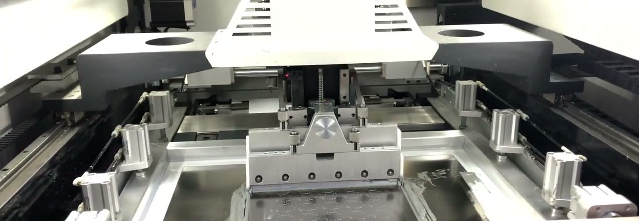
Inside an L5 solder paste printer: the squeegee carriage over the stencil, with paste deposits visible below and pneumatic clamps on both sides. Every OEE factor starts here — the printer is the first station, and its cycle sets the pace for the whole line. Frame from the official JHIMS L5 printer video.
OEE — Overall Equipment Effectiveness — was formalised in the Total Productive Maintenance (TPM) work of Seiichi Nakajima in the 1980s. It is now defined as a key performance indicator in ISO 22400-2, and SEMI E10 covers the equivalent availability metrics for semiconductor manufacturing equipment. The definition is short, and the shortness is the trap: the formula looks complete, but every term in it is a decision you have to make before you calculate.
OEE = Availability × Performance × Quality
Availability = Run Time ÷ Planned Production Time
Performance = (Ideal Cycle Time × Total Count) ÷ Run Time
Quality = Good Count ÷ Total Count
Multiplied out, OEE is simply Valuable Operating Time ÷ Planned Production Time — the share of the time you planned to run that was spent making good product at ideal speed.
Two properties of the formula matter before anything else. First, it multiplies. A line at 90% on all three factors scores 73%, not 90% — and a line that is weak in all three at once is punished three times over. Second, OEE is normally calculated per machine or per line, and the two are different numbers. This article calculates it for the whole SMT line, using the line’s bottleneck cycle as the ideal cycle time. State that choice whenever you quote a figure, because a per-machine OEE and a line OEE answer different questions: per-machine OEE finds the weak station, line OEE tells you what the customer actually receives.
Nakajima grouped the causes of equipment loss into six categories, and each one reduces exactly one of the three factors. The mapping is the whole diagnostic value of OEE: a low score never tells you what to fix, but a low factor does. Here is what each loss looks like on a real SMT line.
| Loss | Factor it reduces | What it looks like on an SMT line |
|---|---|---|
| Breakdowns | Availability | Placement head fault, feeder jam that stops the line, reflow alarm, conveyor fault |
| Setup and adjustment | Availability | Changeover between products: stencil swap, program recall, first-article verification |
| Idling and minor stops | Performance | Board transfer gaps, feeder reload pauses, sensor trips cleared in under a few minutes, waiting for the operator |
| Reduced speed | Performance | Running below the ideal cycle: a conservative profile, worn nozzles, a slower rate on difficult boards |
| Startup rejects | Quality | Boards scrapped or reworked while the process stabilises after a changeover or a cold start |
| Production defects and rework | Quality | Print defects, misplaced parts and solder faults found at SPI, AOI or functional test |
Notice what is missing from the table: there is no row for “the operator was slow” or “the machine is old”. OEE records time, not blame. A feeder jam and a late reel delivery both cost availability; the fix is different, but the factor is the same, and that is why the first step is always to sort losses into the right factor before arguing about causes.
Availability is Run Time divided by Planned Production Time — the time the line was scheduled to run. Breaks, planned maintenance and hours with no orders are not planned production time; they are excluded before the calculation starts. That exclusion is where the gaming begins: every hour you move out of planned time raises availability without the line improving at all.
The three most common moves are easy to recognise once you know them. First, counting changeover as “not planned”. It is planned time — the line was scheduled to run and spent the time changing over. A changeover is a loss inside availability, not an exception to it; our guide to what changeover really costs treats it exactly that way. Second, excluding the first hour after a shift starts as “warm-up”. Third, re-logging a breakdown as “planned maintenance” after the fact. The defence is procedural, not technical: write the planned-time definition down before the week starts, and never change it mid-week.
| Time | Counts as | Why |
|---|---|---|
| Scheduled production hours | Planned production time | The denominator of availability |
| Changeover, stencil swap, program recall | Planned time, lost to setup | The line was scheduled to run; it spent the time changing over |
| Breakdowns, feeder jams, alarms, material starvation | Planned time, lost to breakdowns | Unplanned stops — the line was scheduled to run and did not |
| Meal breaks, planned maintenance, no orders | Not planned time | Excluded before the calculation starts — but fixed in advance, not decided after the fact |
On an SMT line, the unplanned stops worth logging by name are: feeder jams, nozzle pickup errors, stencil cleaning beyond the program, reflow profile alarms, conveyor faults, and material starvation — a reel running out with no splice ready. A stop is unplanned if the line was scheduled to run and it did not, regardless of whose fault it was. Blame does not change the factor, and a stop log that records blame instead of duration is not a measurement tool.
Performance compares actual output with what the line would have produced at its ideal cycle time during the hours it ran. The ideal cycle time is the fastest repeatable cycle for that board on that line — measured, not quoted. Get this one number wrong and the whole factor is fiction.
The classic trap is using a catalogue figure as the ideal cycle. Take the Yamaha YSM40R: it is rated at 200,000 CPH with the 4-beam RS head, at ±0.035 mm accuracy — but that rate is measured under Yamaha optimum conditions, and it is a component-placement rate, not the line’s cycle time for your board. Board transfer, feeder supply and inspection all sit between placements. The YSM40R product page says so plainly: use Yamaha Y.FacT or P-Tool to simulate tact with your specific PCBs before purchase. A line that sets its ideal cycle from a catalogue CPH will report performance below 50% forever and learn nothing — or, more commonly, someone “adjusts” the ideal cycle until performance reads 95%, and the number becomes decoration. The honest ideal cycle is timed on your line, on your board, at steady state.
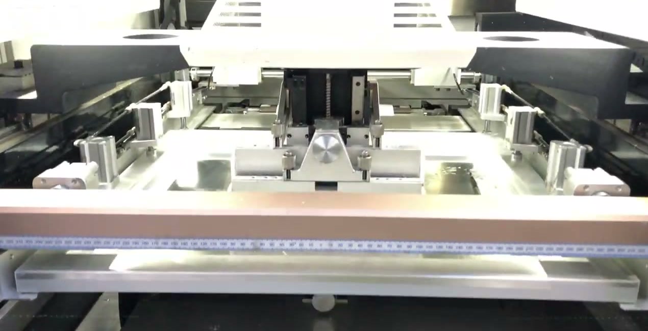
The squeegee carriage of an L5 solder paste printer, seen head-on over the stencil. The print stroke is the printer’s cycle — and the cleaning strokes between prints are part of the real cycle too. Frame from the official JHIMS L5 printer video.
Then there is the quiet killer of performance: micro-stops. Stops under a few minutes — a feeder mis-pick cleared by hand, a sensor trip, a board waiting for the operator — are rarely logged as breakdowns, so they never appear in availability. They appear here, as boards not built. If your line has no stop log, assume micro-stops are your largest performance loss until the log proves otherwise.
The printer shows how the same machine can produce two different ideal cycles. The M8 solder paste printer is published at an 8-second cycle excluding cleaning and 16 seconds including cleaning. Which one is your ideal cycle depends on whether cleaning runs inside the cycle or between boards — and the answer changes the performance factor. State which one you used, in the same document as the OEE figure, or the figure cannot be recomputed by anyone else.
Quality is Good Count divided by Total Count — and “good” means good at first pass. A board that needed rework is not good, even if it eventually ships. Counting reworked boards as good is the most common way to inflate OEE, and it hides the rework bench entirely: the bench keeps working, the factor stops seeing it.
The second quality trap is the startup reject. The first boards after a changeover or a cold start, while the process stabilises, count against quality — not against availability. If your line excludes “warm-up boards” from the count, it is not measuring quality; it is measuring quality after the evidence has been removed.
On an SMT line, quality is decided at three points: printing, placement and reflow. SPI catches print defects first — the S630 3D SPI measures every deposit for volume, area, height, XY offset and shape at 16 µm resolution with Gage R&R under 10%, and feeds corrections back to the printer. AOI checks placement and post-reflow joints. Which station to buy first is a separate decision — our buy-order decision guide for SPI and AOI runs the audit. One boundary to keep clean: first-pass yield (FPY) is the same number as the quality factor when it is measured per board at first pass. This article uses FPY only as the quality leg; tracing a yield drop back to its station is a separate diagnostic with its own method, and it is not rewritten here.
All numbers in this section are illustrative planning numbers. They show the method working; they are not measurements from any real line and not a benchmark. Replace every input with your own timed observations before you use the result.
Assumptions: one 8-hour shift, one product, planned production time 480 minutes. Unplanned stops total 60 minutes — a feeder jam (25), a nozzle pickup error (20) and a reflow temperature alarm (15). The ideal cycle time is 45 seconds per board — the line’s own timed best cycle for this board, assumed for this example. During the run time the line produced 448 boards, of which 430 passed at first pass and 18 failed first pass (12 caught at SPI/AOI, 6 at functional test; all rework-bound or scrapped).
| Step | Calculation | Result |
|---|---|---|
| Availability | Run time 480 − 60 = 420 min; 420 ÷ 480 | 87.5% |
| Performance | (45 s × 448 boards) ÷ (420 × 60 s) = 20,160 ÷ 25,200 | 80.0% |
| Quality | 430 good ÷ 448 produced | 96.0% |
| OEE | 0.875 × 0.800 × 0.960 | 67.2% |
Cross-check: valuable operating time is 430 good boards × 45 seconds = 19,350 seconds = 322.5 minutes. 322.5 ÷ 480 = 67.2% — the same answer by the direct route. If your two routes disagree, one of your inputs is wrong; find it before quoting the number.
Where the time went: of the 480 planned minutes, 157.5 were lost — 60 to availability (the three stops), 84 to performance (420 run minutes minus 336 minutes of ideal-cycle production), and 13.5 to quality (18 failed boards × 45 seconds). The biggest loss is performance, not the visible breakdowns. That is the usual shape, and it is why the three factors must be read separately: the stop log points at the feeder jam, but the money is in the micro-stops nobody logged. And note the gaming arithmetic: if the 18 reworked boards had been counted as good, quality would read 100% and OEE 70% — three points of pure paperwork.
| Move | What it does | How to spot it |
|---|---|---|
| Shrink planned time — exclude changeovers, warm-up, breaks | Availability rises | Ask for the planned-time definition in writing, dated before the measurement week |
| Inflate the ideal cycle time — use a slow “realistic” cycle | Performance rises | Ask how the ideal cycle was timed, on which board, and when |
| Use catalogue CPH as the ideal rate | Performance collapses, then gets “adjusted” upward | Ask for the simulation or the timed cycle behind the number |
| Count reworked boards as good | Quality rises | Ask whether quality is first-pass yield — and check the rework bench is not empty |
| Report the best shift, or the best machine, as “the line” | Everything rises | Ask for the same week, the whole line, every shift |
None of these moves requires dishonesty. Most happen because someone inherited a spreadsheet, changed one definition to make the number “more realistic”, and never wrote the change down. That is why the defence is always the same: the method, in writing, before the measurement starts.
You do not need new software to get a first honest OEE. You need one week and three logs, kept the same way every day.
1. A stop log. Every stop, with start and end time and a reason code taken from the six losses in Section 2. Anything under a few minutes still gets a line — micro-stops are the point, not the exception. A stop with no reason code is a gap in the measurement, not a rounding error.
2. A cycle sample. Time 20 consecutive boards at steady state on each product you run that week. The fastest repeatable time — not the fastest single board, which may be a fluke — is your ideal cycle for that product. Do this per product: a line that runs three boards has three ideal cycles, and one blended number hides all of them.
3. First-pass counts from inspection data. SPI and AOI records already give you first-pass counts without extra paperwork — use them, and do not let anyone reclassify a reworked board as good after the fact.
Three questions to ask any OEE number. (1) What counted as planned time? (2) How was the ideal cycle time set, and for which board? (3) Is the quality factor first-pass yield? If any answer is missing, the percentage is a claim, not a measurement.
Keep the method fixed for at least a month before comparing anything. Changing the ruler mid-month invalidates the trend, and a trend is the only thing OEE is actually good for: is this line better than it was last month, and which factor moved?
OEE can find the bottleneck station: the lowest factor points at the station to fix first, and the loss split in minutes is the improvement budget — 84 minutes of performance loss is a bigger prize than 13.5 minutes of quality loss, whatever the percentages suggest. It can also tell you whether a change worked, provided you compare before and after with the same ruler.
What it cannot do is rank suppliers. Two lines with different boards, different mixes and different rulers produce numbers that cannot be compared — compare scope instead, the way our turnkey quote guide compares it. It cannot set headcount either; that is the staffing method in our operators guide. And it cannot prove a line is “good”. A high-mix line at 67% with six changeovers a day can be a better-run line than a single-product line at 85%.
That last point deserves the 85% benchmark itself. The figure comes from Nakajima’s ideal-plant arithmetic — 90% availability, 95% performance and 99% quality, multiplied to about 85%. It is widely quoted, but it is not a standard, and it assumes a dedicated, continuously running line. A high-mix line will score below it for structural reasons: every changeover is availability lost by design, and every product has its own ideal cycle. Judge a line against its own last month, not against 85%.
No machine raises OEE by itself. A machine removes a specific loss, in minutes, in one factor. That is the test to apply to any effectiveness claim — including ours.
Availability. The Yamaha YSM40R (also listed on jhims.com) attacks the two availability losses directly: the sATS30NS nonstop feeder exchange system reloads tray and tape components without stopping the line, and product changeover takes under 30 seconds with the 128-feeder exchange carriage and automatic program recall, with automatic push-up pin exchange cutting the remaining changeover workload. Those are availability minutes returned to run time — provided the exchange carriage is actually loaded offline before the changeover, which is an operating discipline, not a machine feature.
Performance. The mounter’s catalogue rate is not the line’s rate: 200,000 CPH with the 4-beam RS head, at ±0.035 mm accuracy, is measured under Yamaha optimum conditions. Use Y.FacT or P-Tool to simulate tact with your own PCBs before treating any CPH figure as your ideal cycle. At the printer, the M8 publishes an 8-second cycle excluding cleaning and 16 seconds including it — whether cleaning sits inside the cycle is a program setting, and it changes the performance factor. The machine gives you the cycle; the program decides what counts as one.
Quality. The S630 3D SPI measures every paste deposit and feeds corrections back to the printer, which is how the quality factor stops drifting between shifts. The R10 reflow oven holds ±1°C across 20 independently controlled zones with a 3,840 mm preheating tunnel — profile stability is what keeps first-pass yield from moving with the weather and the shift. Both only help if the quality factor is measured at first pass: an inspection station cannot fix a quality number that counts rework as good.
Limitations, stated plainly. The specifications above are the manufacturers’ published figures for those models, under their stated conditions. They are the inputs to your own OEE calculation, not a promise of an OEE result. Ask which loss, in minutes, a machine removes — and then measure it for a month with the method in Section 8.
Is OEE the same as utilisation?
No. Utilisation compares run time with all calendar time; availability compares it with planned time only. A line can be 100% available and 50% utilised if it has no orders for half the week. The two numbers answer different questions — do not quote one as the other.
Should OEE be measured per machine or per line?
Both are legitimate, but they are different numbers. Per-machine OEE finds the weak station; line OEE is set by the bottleneck and is what the customer actually receives. Never compare one with the other, and say which one you are quoting.
Our line changes over six times a day. Is OEE useless for us?
No — it is more useful, because changeover sits inside availability where you can see it. Expect a lower number than a single-product line, and judge the trend against your own last month rather than against a benchmark built for a dedicated line.
Can I compare my OEE with another factory’s?
Only if the planned-time definition, the ideal cycle and the first-pass rule are identical. In practice they never are. Compare your line with its own last month, with the same ruler.
What is a good OEE for an SMT line?
There is no standard. The widely quoted 85% is Nakajima’s ideal-plant arithmetic (90% × 95% × 99%), not a target. Start by measuring honestly for a month; the first honest number is the baseline, whatever it is.
Bottom line: OEE is Availability × Performance × Quality. Read the three factors, not the product. Ask how planned time was defined, how the ideal cycle was timed, and whether quality is first-pass yield. Fix the lowest factor first — and if the lowest factor is performance, look for micro-stops before buying speed. For specifications, a demonstration on your boards, or a line-effectiveness review, contact JHIMS at [email protected].


 Teams
 whatsapp
 telegram
